Yiling Chen, Debbie Chen
2020 Data Wrangling class final project @ UT Austin ischool
Our project analyzes the possible element that affects The Big Bang Theory viewership. More precisely, we will focus on whether the character relationship or some topic trends seem to impact the number of The Big Bang Theory viewers. This is a whimsical topic, and we hope to demonstrate our data wrangling skills. The viewers' data is organized in Wikipedia, which comes from Nielsen TV Rating, ABC Medianet, etc.
We found data on The Big Bang Theory social network, and it includes each episode from season one to season nine. The analysis will focus on each episode for season 5, and then we will create a pairing name between characters. Next, we will correlate between pairing and the number of viewers. By using this methodology, we can find out the relationship between a couple of characters and the number of The Big Bang Theory viewers.
In addition, we also extract data from Google trends about the topics that may affect the amount of The Big Bang Theory viewers. For example, the topic Star Trek or String Theory are related to The Big Bang Theory and may attract viewers.
Therefore, we will correlate the Google trend data and the number of The Big Bang Theory viewers to find out their relationship.
CSV datasources
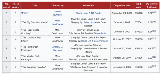
(1) The Big Bang Theory Viewers in Wikipedia
We plan to transfer it use this tool to transform wiki table into .csv
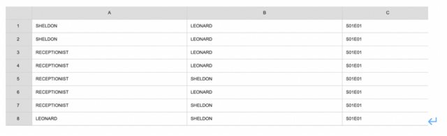
(2) The Big Bang Theory social network
The TBBT social network dataset include two columns of characters: the first column is the speaker, and the second column is the listener. It is a scene association network, where there are many people listening together, and the dataset will record words, like "All", "Women" etc.
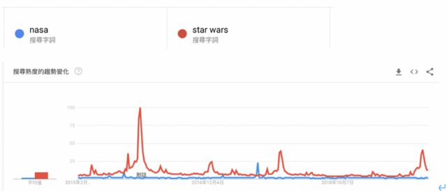
(3) Google trends data with related topic (like NASA, star wars, comic con, string theory, dark matters)
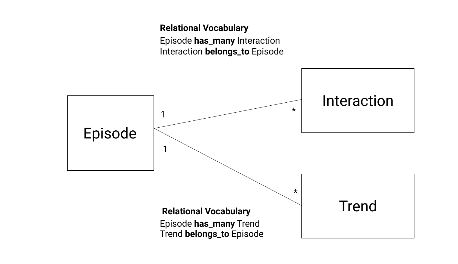
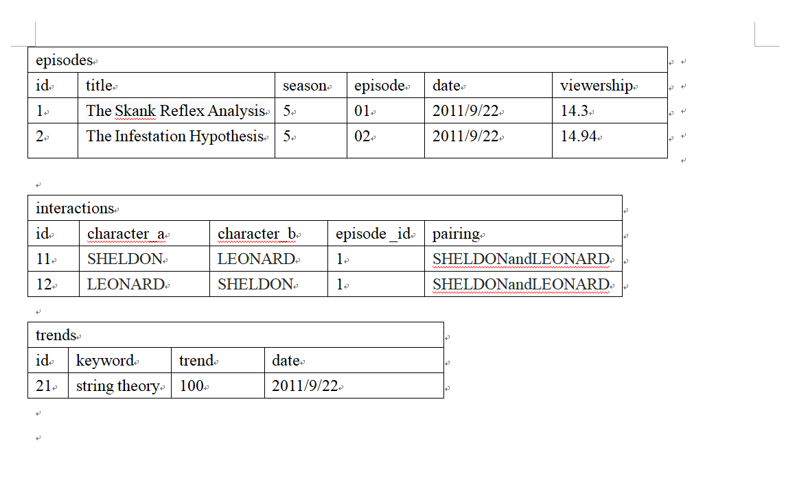
Database Design
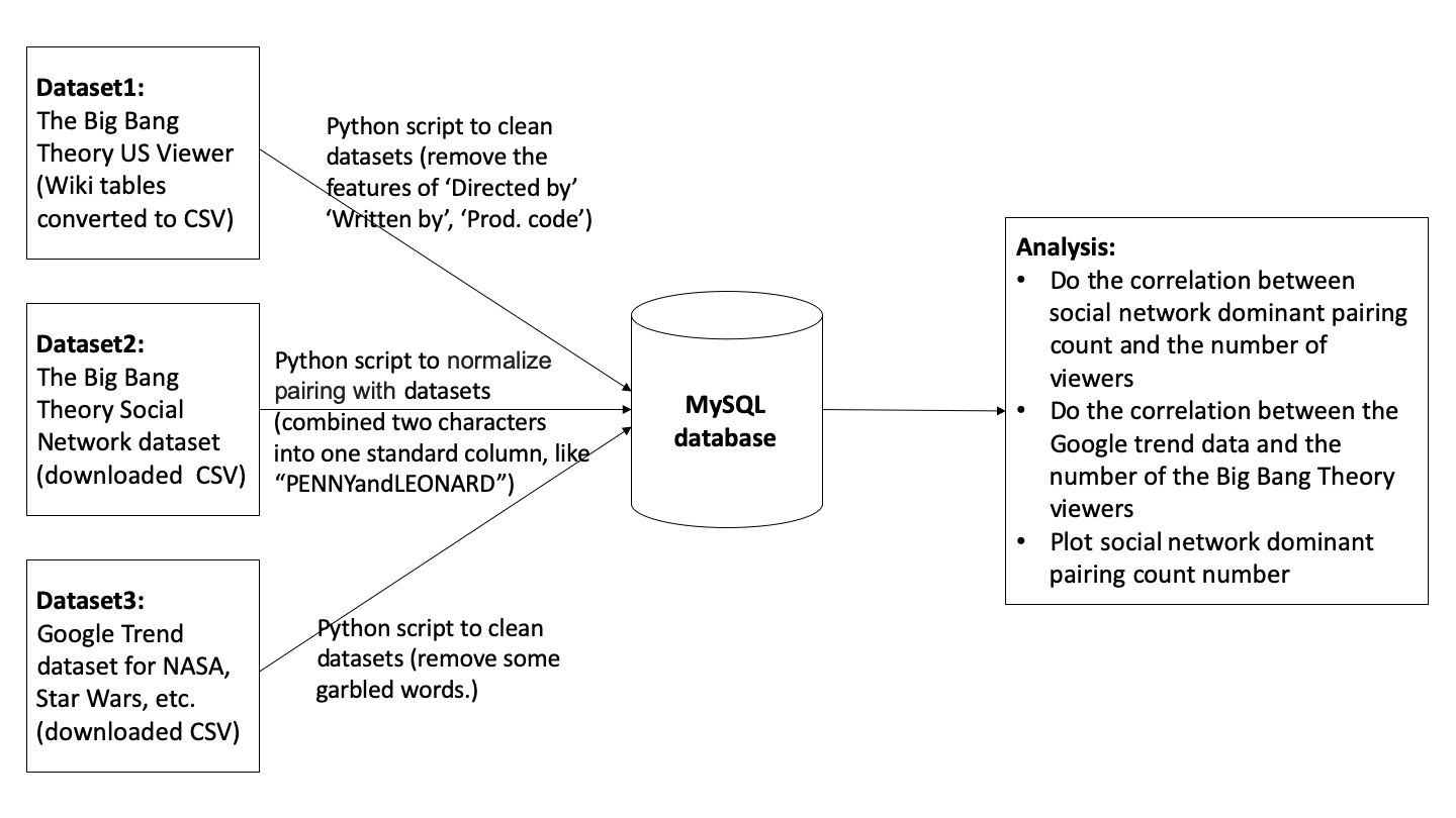
Project Workflow
Load the data into the database
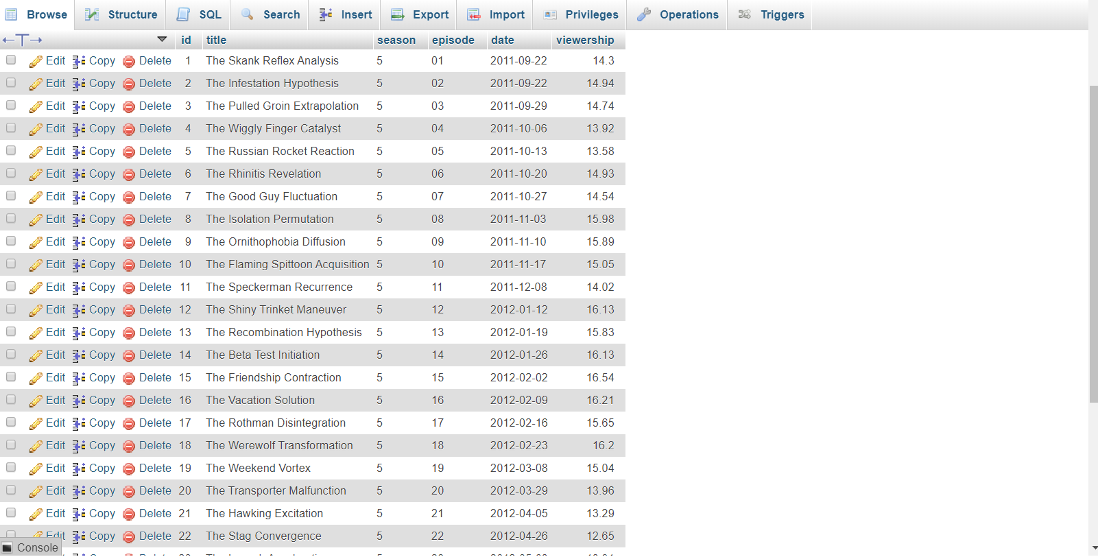
Read TBBT_S5_viewership.csv to episodes table
We inserted the data of each episode for season 5 to episodes table, including title, season, episode, date, and viewership.
#Read TBBT_S5_viewership.csv to episodes table
import csv
import pymysql
import pymysql.cursors
from datetime import datetime

# Set up the connection to the server
connection = pymysql.connect(host="mariadb",
                             user="root",
                             passwd="",
                             db="tbbt",
                             autocommit=True,
                             cursorclass=pymysql.cursors.DictCursor)

# Insert episodes
sql = """
INSERT INTO episodes(title,season,episode,date,viewership)
            VALUE (%(title)s, %(season)s, %(episode)s, %(date)s, %(viewership)s)
"""


with connection.cursor() as cursor:
    with open('TBBT_S5_viewership.csv') as csvfile:
        myCSVReader = csv.DictReader(csvfile)

        # Move row by row through the file
        for row in myCSVReader:
            airdate = row['date']   #Handling dates
            template = "%Y/%m/%d"
            air_datetime = datetime.strptime(airdate, template)  # datetime converts to expected mysql format
            param_dict = {'title': row['title'],
                          'season': row['season'],
                          'episode': row['episode'],
                          'viewership': row['viewership'],
                          'date': air_datetime}

            cursor.execute(sql, param_dict)
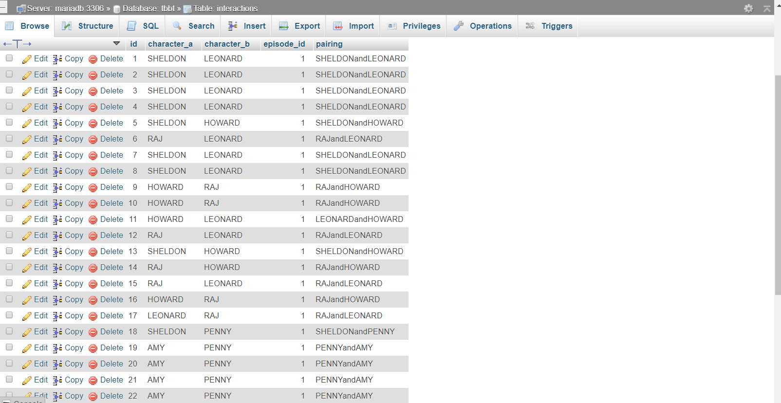
Read network.csv to interactions table
We used the network.csv, and it contained character_a and character_b and episode. We read the network.csv file to insert the data to the database, creating a pairing column in the interactions table. We need to normalize the pair because the pair's name of the first column and second column is the same as the pair's name of the second column and first column. Because we analyzed the data of season 5, we took the data of season 5, getting the episode_id from the episodes table.
#Read network.csv to interactions table
import csv
import pymysql
import pymysql.cursors
from datetime import datetime

# Set up the connection to the server
connection = pymysql.connect(host="mariadb",
                             user="root",
                             passwd="",
                             db="tbbt",
                             autocommit=True,
                             cursorclass=pymysql.cursors.DictCursor)

# Insert interactions
sql = """
INSERT INTO interactions(character_a,character_b,episode_id,pairing) VALUE (%(character_a)s, %(character_b)s, %(episode_id)s, %(pairing)s)
"""


with connection.cursor() as cursor:
    with open('network.csv') as csvfile:
        myCSVReader = csv.DictReader(csvfile)

        # Move row by row through the file
        for row in myCSVReader:
            codedString = row['episode']

            if codedString[1:3] == '05':   #Get the season number that is 05


                character_a = row['character_a']
                character_b = row['character_b']

                #Normalize pairing and create a pairing name

                if(character_a>=character_b):
                    pairingname = f"{character_a}and{character_b}"
                else:
                    pairingname = f"{character_b}and{character_a}"


                codedString = row['episode']
                row['episode'] = codedString[4:6] #Get the episode


                # Use the episode from the row to get the episode_id
                sql_select_episodenum = "SELECT id from episodes WHERE episode = %(episode)s "

                cursor.execute(sql_select_episodenum, row)
                results = cursor.fetchone()
                episode_id = results['id']

                param_dict = {'character_a': row['character_a'],
                              'character_b': row['character_b'],
                              'episode_id': episode_id,
                              'pairing': pairingname}

                cursor.execute(sql, param_dict)
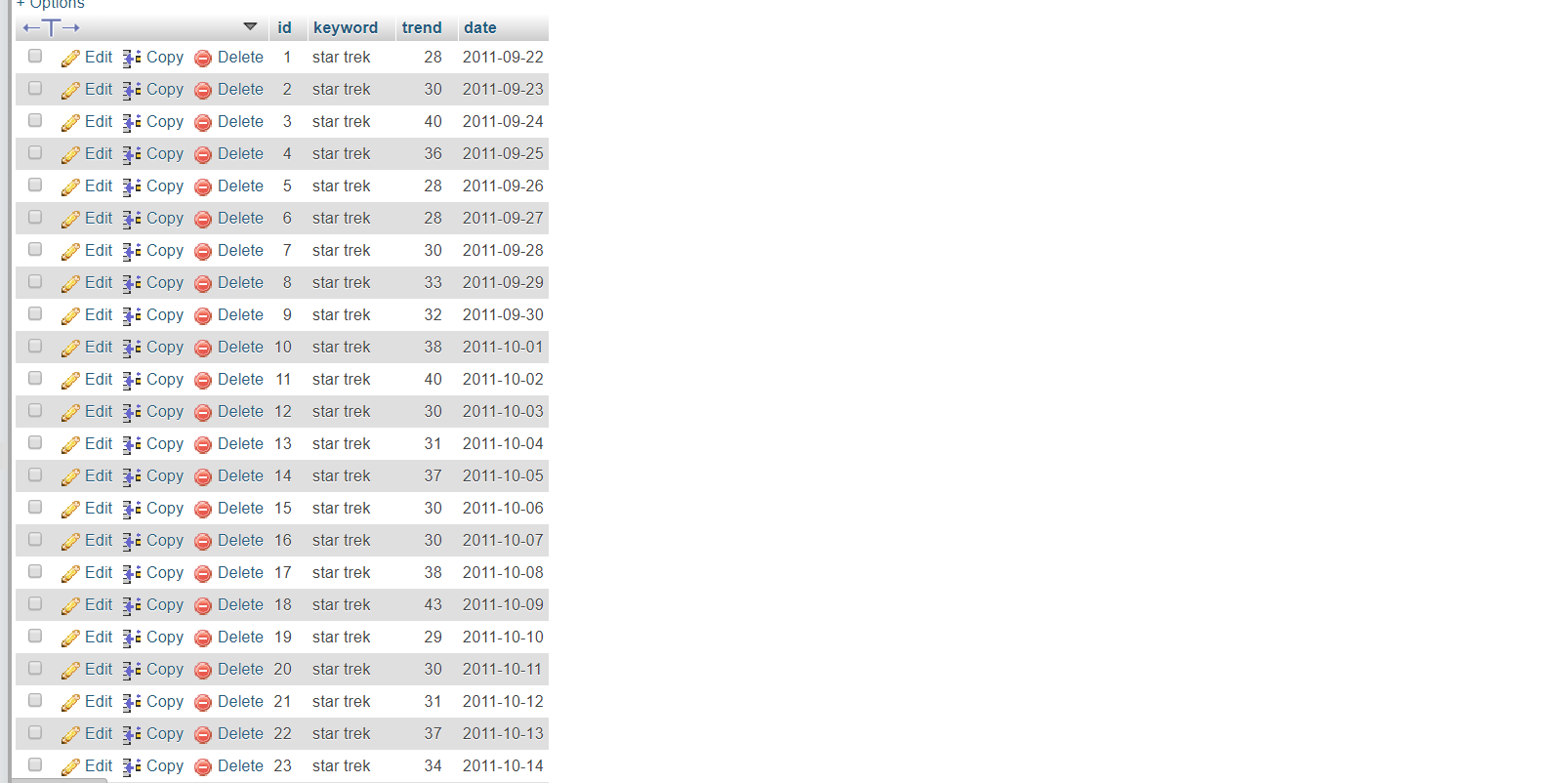
Read string theory_trend.csv, star trek_trend.csv, comic con_trend.csv to trends table
Following is the code for inserting the data of string theory_trend.csv to the trends table. We used the same code for reading star trek_trend.csv and comic con_trend.csv; only the filenames are different.
#import trends data
import csv
import pymysql
import pymysql.cursors
from datetime import datetime
import re
# Set up the connection to the server
connection = pymysql.connect(host="mariadb",
                             user="root",
                             passwd="",
                             db="tbbt",
                             autocommit=True,
                             cursorclass=pymysql.cursors.DictCursor)

# Insert trends
sql = """
INSERT INTO trends(keyword,trend,date) VALUE (%(keyword)s, %(trend)s, %(date)s)
"""

with connection.cursor() as cursor:
    with open('string theory_trend.csv') as csvfile:
        myCSVReader = csv.DictReader(csvfile)

        #Get the keyword from the file name
        filename = "string theory_trend.csv"
        matches = re.search('(.+)_(.+)',filename)
        keyword=matches.group(1)

        # Move row by row through the file
        for row in myCSVReader:
            trenddate = row['date']
            template = "%Y/%m/%d"
            trend_datetime = datetime.strptime(trenddate, template)  # datetime converts to expected mysql format

            param_dict = {'keyword': keyword,
                          'trend': row['trend'],
                          'date': trend_datetime}

            cursor.execute(sql, param_dict)
Result (Statistic, Graph)
In the result part, we will focus on two analysis.
The first one is that we will use Tableau to draw some graphs to demonstrate our dataset.
The second thing is that we will use Python to calculate their correlation between US Viewship, social network, and google trend.
Query the tbbt database to output to a file called "pairingandviewer.csv" and "trendandviewer.csv". Then read the CSV to analyze the data.
with connection.cursor() as cursor:
    # SQL queries are just a string.
    sql = "SELECT interactions.pairing as pairing, interactions.episode_id as episode_id,episodes.viewership as viewership FROM interactions JOIN episodes ON interactions.episode_id=episodes.id"
    cursor.execute(sql)
    results = cursor.fetchall()  # list of dicts

    # examine query and results
    print(sql)
    print(results) # see, a list of dicts

with open('pairingandviewer.csv', 'w') as csvfile:
    column_names = list(results[0].keys()) #  or manual list
    myCsvWriter = csv.DictWriter(csvfile,
                                 fieldnames = column_names)

    myCsvWriter.writeheader()

    # write the rows. We iterate through results.
    for row in results:
        myCsvWriter.writerow(row)

print("Done writing csv")
with connection.cursor() as cursor:
    # SQL queries are just a string.
    sql = "SELECT trends.keyword as keyword,trends.trend as trend,episodes.id as episode_id, episodes.viewership as viewership FROM trends JOIN episodes ON trends.date=episodes.date"
    cursor.execute(sql)
    results = cursor.fetchall()  # list of dicts

    # examine query and results
    print(sql)
    print(results) # see, a list of dicts

with open('trendandviewer.csv', 'w') as csvfile:
    column_names = list(results[0].keys()) #  or manual list
    myCsvWriter = csv.DictWriter(csvfile,
                                 fieldnames = column_names)

    myCsvWriter.writeheader()

    # write the rows. We iterate through results.
    for row in results:
        myCsvWriter.writerow(row)

print("Done writing csv")
Data Visualization
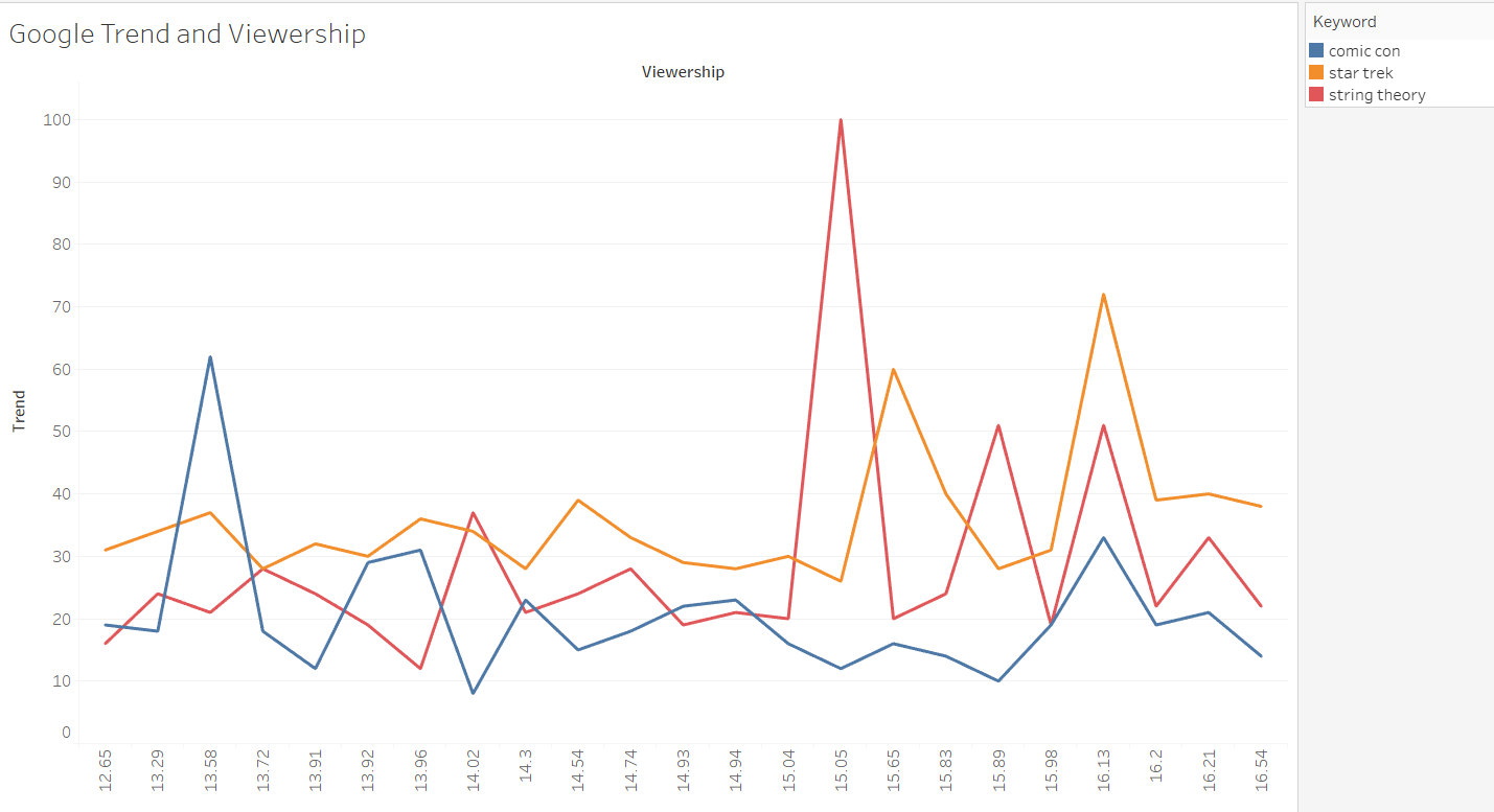
Google Trend and Viewership
We first use Tableau to visualize our dataset. Sorting by the viewership, we plot our Google Trend dataset based on different keywords.
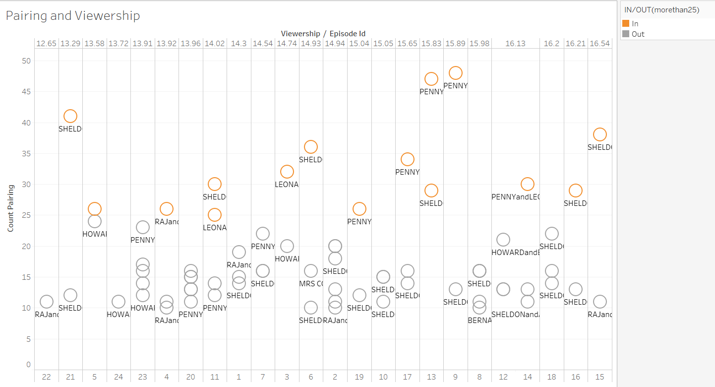
Pairing and Viewership
The X-axis is a sorting viewership, and the Y-axis is the number of how many times these pairs interact. We only selected those pairs that have shown more than 10 times, and we use different colors to highlight those pairs that have shown more than 25 times.
Correlation
The relationship between Social Network and Viewership
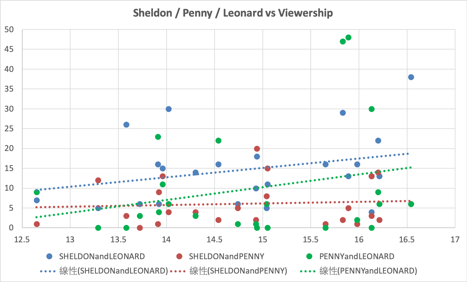
To analyze the relationship between social network and viewership, we first calcuate the number of pairing in each episode. After we got the count value of the dominant pairing, we picked two important relationship to calculate the correlation.
The first vital social network in the TBBT is the relationship between Sheldon, Leonard and Penny. To see how will the social network affect viewership, we plot scatter plot and caculate the correlation value to determine the result. As the table showed, we can see all three social network is positive correlation. In addition, when the number Sheldon&Leonard is higher, it may caused more viewership.
| Sheldon&Leonard | Leonard&Penny | Sheldon&Penny |
|---|---|---|
| 0.2924 | 0.2510 | 0.0778 |
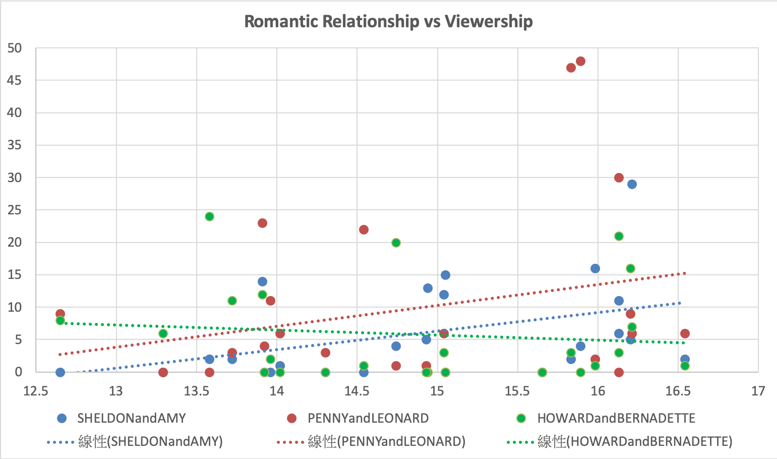
The second crucial social network is the romantic relationship between the characters. Therefore, we picked three dominant romantic relationship in the TBBT. Based on the table and the scatter plot below, we can see Sheldon&Amy and Leonard&Penny can really help viewshipe higher. However, the Howard&ernadette and the viewership is negative correlation, which means when Howard&ernadette appears more, the viewership may decrease.
| Sheldon&Amy | Leonard&Penny | Howard&ernadette |
|---|---|---|
| 0.4259 | 0.2510 | -0.1133 |
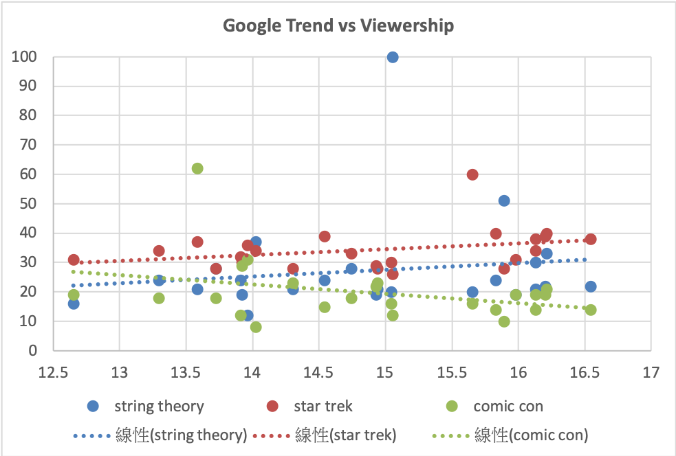
The relationship between Google Trend and Viewership
In terms of the relationship between specific keywords of Google Trend and Viewership, we also did the correlation to examine the result. Based on our chosed keywords, we can see there are some correlation between them. For example, the Star Trek and String Theory have a positive correlation with Viewership. On the other hand, the Comic COn and the Viewership has a negative correlation.
| Star Trek | String Theory | Comic Con |
|---|---|---|
| 0.3146 | 0.1444 | -0.3311 |
Resolving Challenges
One of the most challenging parts was to deal with the social network dataset. First, we considered creating a network graph; however, it was not easy for us to figure out how to do it. We decided to find the dominant pairs for the episodes since the data contains the speaker (first column) and the listener (second column) of each dialogue line. A second challenge was to create the same name of the pair in both the first column and second column. After seeking help, we learned how to create and normalize pairing by ordering the character name in a consistent way. Following are the code we used:
if(character_a>=character_b):
pairingname = f"{character_a}and{character_b}"
else:
pairingname = f"{character_b}and{character_a}"
Also, the third column contains both seasons and episodes; we had to split the data out to get what we want. To do this, we chose start_pos and end_pos to get the season and episodes. Because we only analyzed the data of season 5, we used if statement to get the data of season 5. In addition, after getting the episodes, we used SELECT id from the episode's table to get the episode_id.
We read the course material and followed it step by step. It was not easy for us to combine all of these techniques at the same time. The error messages shown after running the cells also made us frustrated, but we learned a lot by debugging, by searching for help online and by experimenting with different techniques. When we inserted the CSV file successfully, we were really delighted.
Learning an Analysis Tool
One of the analysis tools I learned is Tableau, and I learned how to use it from the course data storytelling I took this semester. I was glad to have the opportunity to use this tool in different classes. When I first learned how to use Tableau, the professor encouraged us to explore how to present the data in various ways. Therefore, I usually linked the data to a CSV file and then tried different methods to visualize the data. Sometimes I might not achieve the result I expected at first, but I got a better visualization during the exploration. Besides the data visualization course, this data wrangling course was also helpful for me to learn Tableau. For example, I understood more about Tableau after taking the class on the pivot table. Besides the course, I also watched online teaching videos of Tableau or browsed Tableau Public Gallery to get more inspirations. To do better analysis, I want to keep exploring Tableau and find out more about it in the future.